\(\Im\in\int\int\)

deep learning worked

This document covers the foundations of neural networks by training one in a fullstack fashion from math to metal. We will build a deep learning framework from scratch starting with the tensor frontend, autodiff engine, supporting both CUDA and Triton.

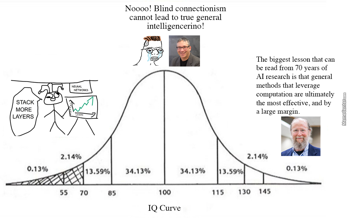
Why neural networks? bitter lesson. compositionality. representation learning.

universal behavioral cloner (universal function approximation)

representation

optimization

In deep learning most learning methods are gradient-based, since the core problem is one of parameter estimation, solved by \[ \boldsymbol{\theta}^* = \underset{\boldsymbol{\theta} \in \Theta}{\operatorname{argmin}} \mathcal{L}(\boldsymbol{\theta}) \] where \(\mathcal{L}: \Theta \mapsto \mathbb{R} \), and \(\operatorname{argmin}\) is implemented iteratively with gradient descent: \[ \boldsymbol{\theta}_{i+1} = \boldsymbol{\theta}_i - \alpha \nabla_{\boldsymbol{\theta}} \mathcal{L}(\boldsymbol{\theta}_i) \]

Now that we have formalized the "goodness" of our neural network's parameter (weights and biases) estimation with the loss function \(\mathcal{L}: \Theta \mapsto \mathbb{R} \) defined as ____, we will now perform parameter estimation with the following optimization problem: \[ \boldsymbol{\theta}^* = \underset{\boldsymbol{\theta} \in \Theta}{\operatorname{argmin}} \mathcal{L}(\boldsymbol{\theta}) \] where \(\operatorname*{argmin}\) is implemented with automatic differentiation. To motivate the algorithmic nature of automatic differentiation, let's take a look at symbolic and numeric differentiation first.

This optimization problem is typically solved using iterative methods, most commonly variants of gradient descent. The basic idea is to update the parameters in the direction of steepest descent:

\[\theta_{t+1} = \theta_t - \alpha \nabla f(\theta_t)\]

where \(\alpha\) is the learning rate and \(\nabla f(\theta_t)\) is the gradient of \(f\) at \(\theta_t\).

The challenge in neural network optimization lies in the high-dimensionality of the parameter space, the non-convexity of the loss landscape, and the need for efficient computation of gradients, which is addressed by backpropagation and automatic differentiation.

generalization

on generalization... Because we are approximating population loss with sample loss, there are times where we perform well on the computable sample loss yet perform poorly on population loss (approximated further by evaluating our predictor on unseen data from the underlying data generating distribution). This can happen due to a lack of data (underfitting), or due to an excess of model complexity (overfitting). Both of them leads to poor generalization on the population loss.

• Nielsen 2015
• Goodfellow et al 2016
• Prince 2023