\(\Im\in\int\int\)
appendix
This appendix is a condensed summary of the half-learned concepts retained during my symbol-bashing undergraduate days studying mathematics, which is a universal code library maintained for centuries with no versioning and no central maintainers. Surprisingly, the maths to understand machine learning at an operational level are quite mundane, and most of it is simply a more formalized notion of the math you learn in high school.
The descriptive syntax I use for denotation is the same that maths and physics have checked out last century, using notions involving infinities such as real numbers, limits, and integrals, even though the connotation of implementation I hold in my head are potentials for me to approximate and compute, rather than actuals I can hold. We will define notions both
- mathematically, by describing what objects do, with general axioms in order to avoid commiting to internal structure, which allows for a much broader class of objects to be considered
- computationally, by describing what objects are, with the representation of the internal structure encoded by a turing machine or lambda calculus, which allows for the objects to be computable
In mathematics, most areas deal with various types of spaces and study
- functions defined between those spaces
- how these functions perserve or do not perserve various properties of these spaces.
probability
Probability theory gives us a way to quantify and represent uncertainty around stochastic (non-deterministic) phenomena by distributing truth across a weighted set of events. Laplace said it best: probability is common sense reduced to calculus.
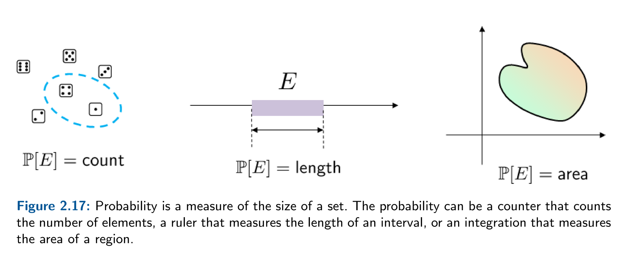
Formally, we represent a probability space with a triplet \(({\Omega}, \mathcal{F}, \mathbb{P})\), where \(\Omega\) is the sample space of, \(\mathcal{F}\) is the event space, and \(\mathbb{P}\) is a measure \(\mathcal{F} \mapsto [0,1]\). In practice, this probability space is implicit, but establishing this mathematical machinery helps us be very explicit with what notions we are formalizing. A probability space allow us to
- decouple the measurer from the measurable space
- decouple the probability assignment from the underlying event
The first decoupling allows for different spaces and measurers very naturally: counters, and integrators. The second decoupling allows naturally gives rise to both frequentist and bayesian perspectives depending on the availability of data.
The axioms of probability are an extension of deductive logic, and there's only three:
- \(\mathbb{P}(A) > 0 \)
- \(\mathbb{P}(\Omega) = 1 \)
- \(\mathbb{P}(A \cup B) = \mathbb{P}(A) + \mathbb{P}(B)\) if \(A\) and \(B\) are mutually exclusive
TODO: bayes theorem is a more general version of aristotle's syllogism
The first two axioms are pretty easy to accept. Other possible ways of defining a formal representation to capture uncertainty will look similar, perhaps with different numbers which encode our intuitions around impossible and guaranteed events.
The third axiom formally captures our intuition around adding probabilities of two events when there's no overlap. This can be extended for \(n\) events so that if \(A_1, A_2, \ldots, A_n\) are mutually exclusive events, then \[ \mathbb{P}(A_1 \cup A_2 \cup \cdots \cup A_n) = \sum_{i=1}^n \mathbb{P}(A_i) \] which we call the sum rule.
Conditional, independance, product rule
Once we have the three axioms of probability defined, we can build compound notions such as conditional probability, which is the probability of event \(A\) after seeing event \(B\). \[ \mathbb{P}(A|B) := \frac{\mathbb{P}(A \cap B)}{\mathbb{P}(B)} \] which algebraically captures the intuition from drawing out the sets \(A\) and \(B\) — the conditional probability should be the ratio of the area of set \(A\) relative to the area of set \(B\).
Following our intuition from the visualization of the two sets, if the set \(A\) has no overlap with the set \(B\), then the equation for the conditional probability above should evaluate to \(P(A)\), which means \(P(A \cap B) = P(A)P(B)\). This relationship forms the definition for the independance of two events.
Finally, we can use our relationship for conditional probability to rearrange for \(\mathbb{P}(A \cap B)\), \[ \mathbb{P}(A \cap B) = \mathbb{P}(B)\mathbb{P}(A|B) \] which seems like a useful identity to use when we want to evaluate for the probability that both events happen, and we know the terms on the right hand side. We'll call this particular rearrangement of conditional probability the chain rule or product rule. We can extend the chain rule for \(n\) events: \[ \mathbb{P}(A_1 \cap A_2 \cap \cdots \cap A_n) = \mathbb{P}(A_1)\mathbb{P}(A_2|A_1)\mathbb{P}(A_3|A_1,A_2)\cdots\mathbb{P}(A_n|A_1,\ldots,A_{n-1}) \] and when the events are independant, we can evaluate the left hand side with: \[ \mathbb{P}(A_1 \cap A_2 \cap \cdots \cap A_n) = \prod_{i=1}^n \mathbb{P}(A_i) \]
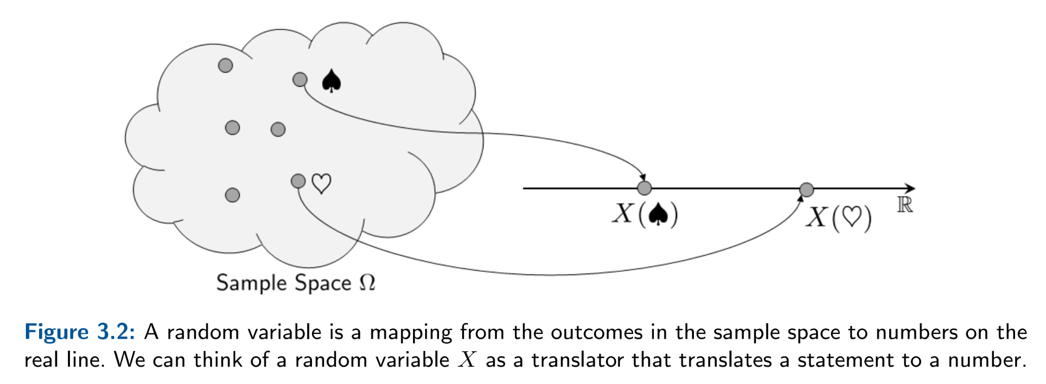
However, in practice, we forget about the probability space and probability measures taking in events (of type set) by using discrete random variables \(X:\Omega \mapsto \mathbb{N} \) and continuous random variables \(X:\Omega \mapsto \mathbb{R} \) in order to map sets over to the natural and real number lines. This lets us define idealized notions such as expectation, variance, and their computable estimators. Like computer science, the term random variable is a misnomer for what the object's true type really is: a mapping. Once we have random variables, we summarize all mapped events with a probability distribution.
Discrete random variables
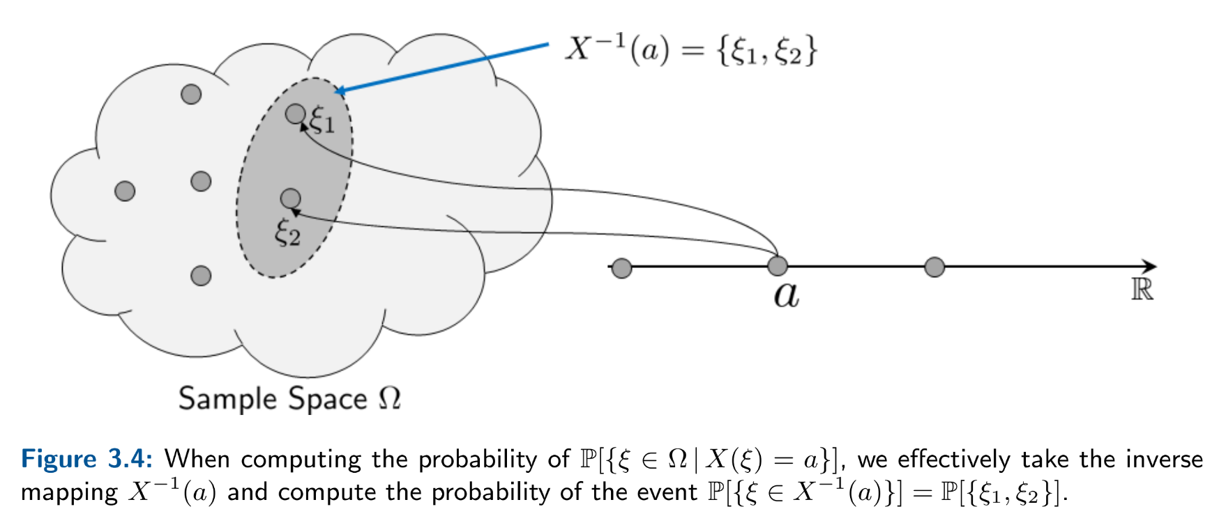
When the measurable space is discrete and the measurer \(\mathbb{P}\) is a counter, we call the random variable discrete, and the resulting distribution a probability mass function \( p_X: Im(X) \mapsto [0,1] \) where \(p_X(x) := \mathbb{P}[X=x]\). So, when evaluating the probability of an event \(A\), \begin{align*} \sum_{x \in A} p_X(x) &= \mathbb{P}[X \in A] \\ &= \mathbb{P}[X^{-1}(A)] \\ &= \mathbb{P}[\{\omega \in \Omega: X(\omega) \in A \}] \\ &= \mathbb{P}[A] \end{align*} We can extend the function to support two random variables so that \( p_{X,Y}: \mathbb{R} \times \mathbb{R} \mapsto [0,1] \) where \(p_{X,Y} := \mathbb{P}[X=x, Y=y] \). So, when evaluating the probability of an event \(A\), \begin{align*} \sum \sum_{(x,y) \in A} p_{X,Y}(x,y) &= \mathbb{P}[(X,Y) \in A] \\ &= \mathbb{P}[(X,Y)^{-1}(A-0-=)] \\ &= \mathbb{P}[\{(\omega_1, \omega_2) \in \Omega \times \Omega: (X(\omega_1), Y(\omega_2)) \in A \}] \\ &= \mathbb{P}[A] \end{align*} and for \(n\) random variables we have Regardless of type, the pmf needs to total up to 1 (\(\sum_{x \in Im(X)} p_X(x) = 1\)) which is a direct result of axiom 2.
Continuous random variables
When the measurable space is continuous and the measurer \(\mathbb{P}\) is an integrator, we call the random variable continuous, and the resulting distribution a probability density function \( f_X: Im(X) \mapsto [0,\infty) \) where \(f_X(x) := \frac{d}{dx}F_X(x)\), and \(F_X(x) = \mathbb{P}[X \le x]\).
The reason why the pdf is defined this way is because the uncountable space forces us to define the measurer as an integrator. If we measured the function at a single point, it would evaluate to zero: \( \int_a^a f_X(x) dx = 0\), so it would be incorrect to define \(f_X(x) := \mathbb{P}[X=x]\). Thus, we define the function to be the derivative of the cdf, which we integrate in order to evaluate probabilities. This is why the function is called a probability density function, for it returns the probability per unit length. Finally, when evaluating the probability of an event \(A\), \begin{align*} \int_{x \in A} f_X(x) dx &= \int_a^b f_X(x) dx \\ &= \mathbb{P}[a \le X \le b] \\ &= \mathbb{P}[A] \end{align*} for two random variables we have \begin{align*} \int \int_{(x,y) \in A} f_{X, Y}(x, y) d{x}d{y} &= \int_c^d\int_a^b f_{X,Y}(x,y) d{x}d{y} \\ &= \mathbb{P}[a \le X \le b, c \le Y \le d] \\ &= \mathbb{P}[A] \end{align*} and for \(n\) random variables we have Like the discrete case, regardless of type, the pdf needs to total up to 1 (\(\int_{-\infty}^{\infty} f_X(x) dx = 1\)) which is a direct result of axiom 2.
Notions of conditions, chain rule, and independance also carry over to random variables from events. We say random variables \(X_1\) and \(X_2\) are independant if and only if \(p_{X_1,X_2} = p_{X_1}(x_1)p_{X_2}(x_2)\), which follows directly from the definition of independance on events. All definitions can be extended to the general case where we have random variables \(X_1,...,X_N\).
x-ray: sum rule, product rule, chain rule, bayes rule independance defined by conditional?
Expectation, variance, covariance
Distributions that sum/integrate to 1 with interesting stories — \(Ber(p)\), \(Poi(\lambda)\), \(Uni(\alpha, \beta)\), \(Nor(\mu, \sigma)\). and go over their expectations and variances...
Law of large numbers, central limit theorem
Referenceslinear algebra
Vector spaces and bases
Linear algebra gives us a way to represent linear transformations in vector spaces and talk about their algebraic properties. This means that the field is concerned with equating objects, rather than counting like combinatorics or approximating like analysis.
Algebraically, we represent a vector space with a quadruplet \((V, \mathbb{F}, +, \cdot)\), where \(V\) is a set of vectors, \(\mathbb{F}\) is a field of scalars (typically \(\mathbb{R}\) or \(\mathbb{C}\)) equipped with two operations: 1. an inner operation \(+: V \times V \mapsto V \) called vector addition and 2. an outer operation \(\cdot : \mathbb{F} \times V \mapsto V\) called scalar multiplication.
The vectors in the vector space satisfy the laws of algebra such that \(V\) is closed under vector addition and scalar multiplication. todo: neutral elements (0 and 1)
Computationally, we a can represent vectors as mappings. For instance, a vector \(\mathbf{x} \in \mathbb{R}^d\) can be represented as a function where \(\mathbf{x}: \{0, 1, ..., d-1\} \to \mathbb{R}\). With this representation, vectors map position to space — this representation admits a labelling scheme interpretation, which we call a coordinate system. This representation admits the interpretation of linear algebra as a generalized form of Cartesian coordinate geometry in \(d\) dimensions.
Regardless of representation, the core operation within vector spaces is the linear combination. It's a compound expression where both vector addition and scalar multiplication are used to express one vector in terms of others: \[ \begin{align} \mathbf{y} &= \alpha_1\mathbf{x}_1 + \alpha_2\mathbf{x}_2 + \cdots + \alpha_n\mathbf{x}_n \\ &= \sum_{i=1}^n \alpha_i\mathbf{x}_i \end{align} \]
A natural question to then ask is what vectors \(\mathbf{y}\) can be produce with the set of vectors \(\{\mathbf{x}_1, \mathbf{x}_2, \ldots, \mathbf{x}_n\}\). This set of all possible linear combinations is called the span, where \( \text{span}(\{\mathbf{x}_1, \mathbf{x}_2, \ldots, \mathbf{x}_n\}) = \left\{\sum_{i=1}^n \alpha_i\mathbf{x}_i : \alpha_i \in \mathbb{F}\right\} \).
a basis is a spanning set which is independant
dimension..
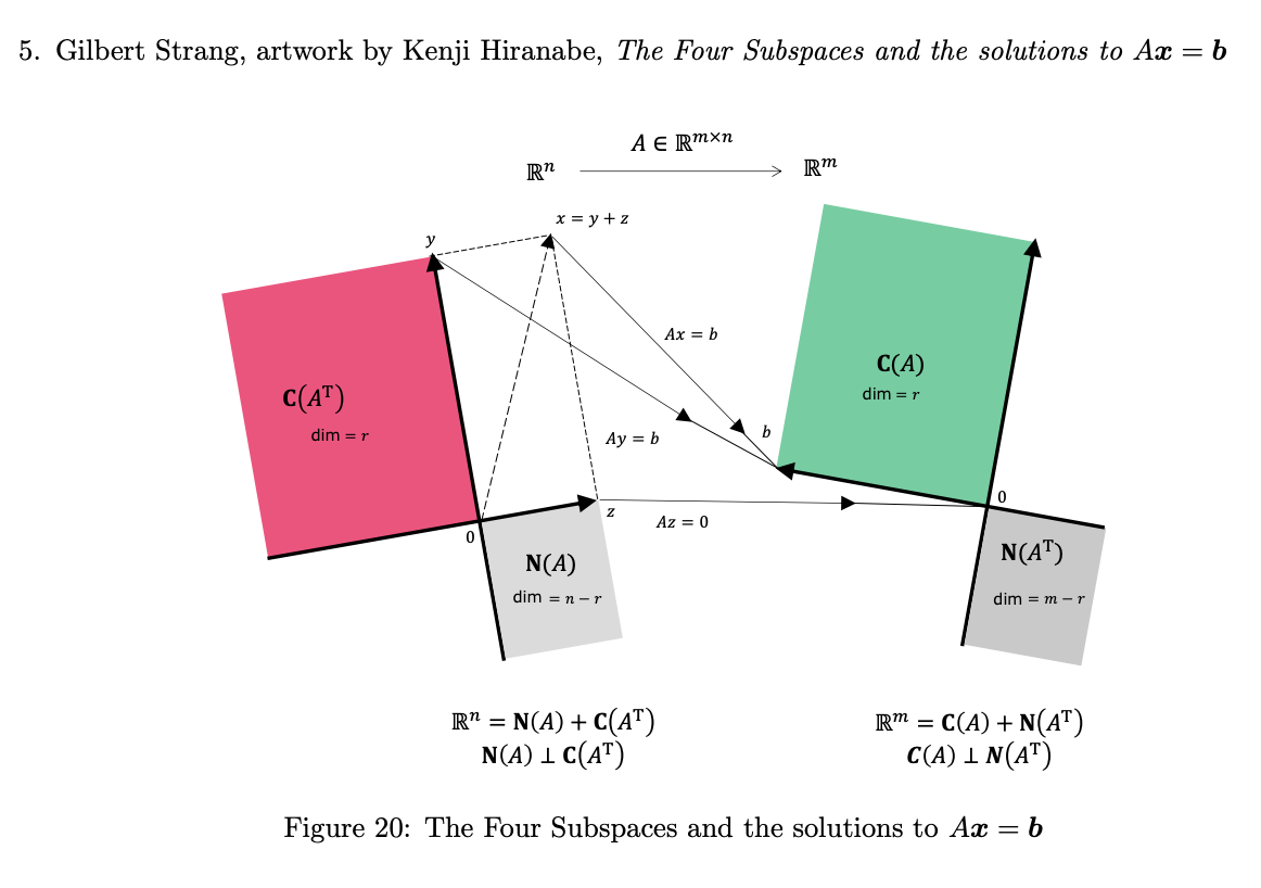
Linear transformations: matrices, four subspaces, determinant, trace
The core of linear algebra is the linear transformation which is encoded with a matrix: \[ \mathbf{A}\mathbf{x} = \mathbf{b} \] where \(\mathbf{A} \in \mathbb{R}^{n \times d}\), \(\mathbf{x} \in \mathbb{R}^d\), and \(\mathbf{b} \in \mathbb{R}^n\). We can then define some function \( f: \mathbb{R}^d \mapsto \mathbb{R}^n \) where \( f := \mathbf{A}\mathbf{x}\).
For efficient computation, it's best to view matrix vector multiplication from the row-oriented perspective, in which each entry of the result is the inner product \(A\)'s rows with \(\mathbf{x}\) \[ \begin{bmatrix} 1 & 2 & 0 \\ -5 & 3 & 1 \end{bmatrix} \begin{bmatrix} 0 \\ 1 \\ 0 \end{bmatrix} = \begin{bmatrix} 0(1) + 1(2) + 0(0) \\ 0(-5) + 3(2) + 1(0) \\ \end{bmatrix} = \begin{bmatrix} 2 \\ 3 \end{bmatrix} \]
For understanding how matrices encode linear transformations, it's best to look at the mechanics of matrix vector multiplication from the column-oriented perspective. For example: \[ \begin{bmatrix} 1 & 2 & 0 \\ -5 & 3 & 1 \end{bmatrix} \begin{bmatrix} 0 \\ 1 \\ 0 \end{bmatrix} = 0\begin{bmatrix}1 \\ -5\end{bmatrix} + 1\begin{bmatrix}2 \\ 3\end{bmatrix} + 0\begin{bmatrix}0 \\ 1\end{bmatrix} = \begin{bmatrix} 2 \\ 3 \end{bmatrix} \] You can see that the first step in evaluating the matrix vector multiplication is to map over the \(d\) entries of \(\mathbf{x}\) by multiplying them with the \(d\) column vectors of \(A\). The second step is to evaluate the linear combination of the \(d\) column vectors into a single vector \(\mathbf{b} \in \mathbb{R}^n\). Fundamentally, \(\mathbf{A}\mathbf{x}\) is a linear combination of the columns of \(\mathbf{A}\).
The perspective of matrix vector multiplication as a linear combination of a matrix's columns connects matrices back to notions of vector spaces. four foundamental spaces..
four fundamental subspace. dimension..rank..pivot columns..basis.. applied to matrices
All transformations we care about are linear. Using geometry as an intuition, this means transformations such as scaling, rotation, reflection, and shearing.
Matrix-matrix multiplication can be seen as an extension to this, where instead of mapping over a single vector, we map over multiple vectors, which in turn, forms a matrix (that encodes a linear transformation itself). Matrix multiplication is function composition..
transformations...
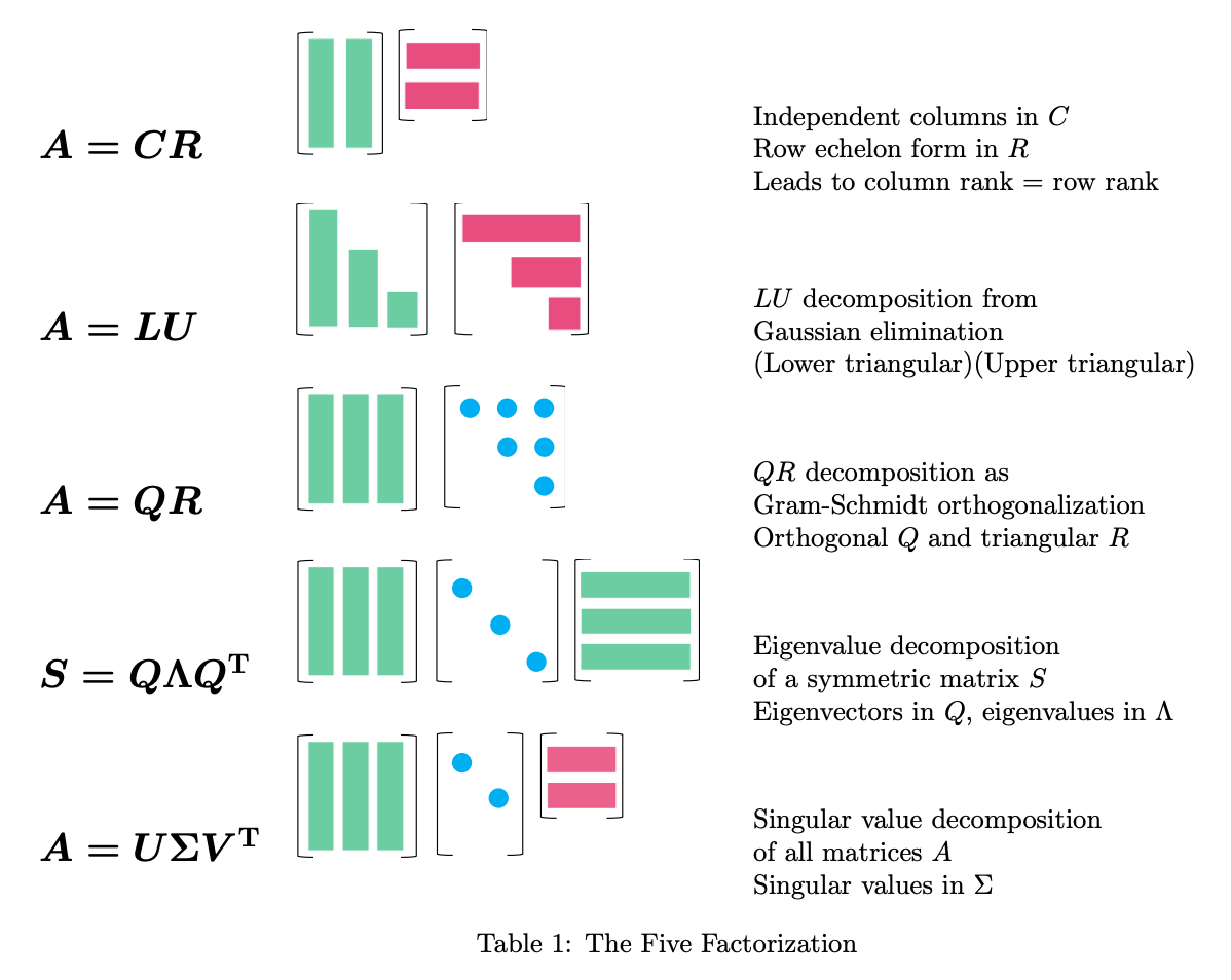
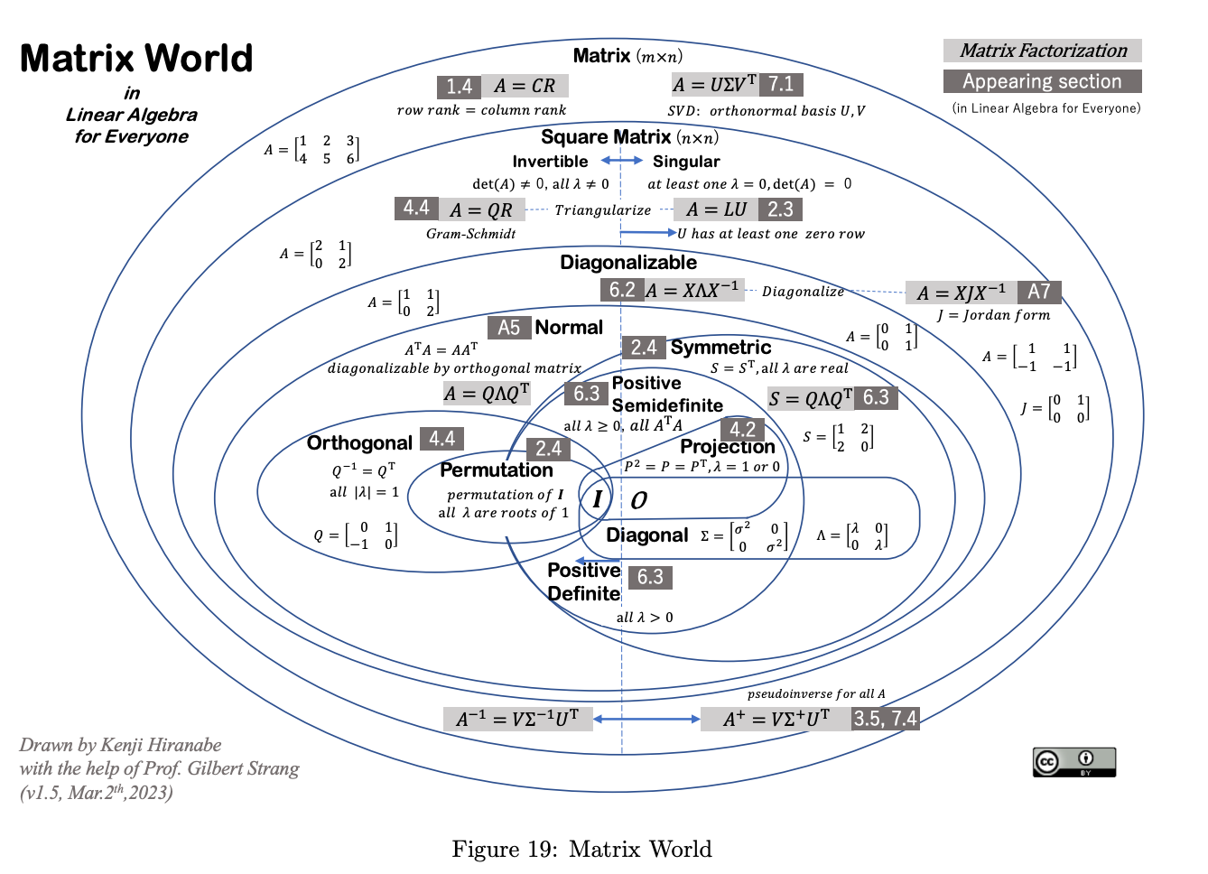
we will now cover the primary decompositions..
Analytic geometry: length, distance, angle
Inner products..
Length and distance..
Angles and orthogonality..
Orthogonal vectors
\(A = QR\)
Eigenvectors
\(A = Q\Lambda Q^T\)
Singular vectors
\(A = U\Sigma V^T\)
Referencesoptimization
Optimization theory gives us a way to represent what our optimal aspirations are: to minimize risk, maximize reward, reduce energy consumption, etc. Most continuous optimization methods use differential calculus, the core tool being the instantaneous rate of change of some function with respect to its inputs.
Univariate optimization:\(\, \frac{df}{dx}\)
For some function \(f: \mathbb{R} \mapsto \mathbb{R} \), we can approximate the rate of change over some interval with \[ \frac{\Delta f}{\Delta x} := \frac{f(x + \Delta x) - f(x)}{\Delta x} \] and to figure out the behavior of the function near a single "point", we can take the definition above, let the interval approach zero, and denote this infinitesimal behavior with \(\frac{d}{dx}: (\mathbb{R} \to \mathbb{R}) \to (\mathbb{R} \to \mathbb{R})\), calling it the derivative of f with respect to x: \[ \frac{df}{dx} := \lim_{\Delta x \to 0} \frac{f(x + \Delta x) - f(x)}{\Delta x} \] This operator takes a differentiable function (the limit exists) and maps it over to its derivative function. The limit of the input expression above exists when ...
Multivariate optimization:\(\, \nabla f\)
We can extend this notion to support functions of multiple variables \(f: \mathbb{R}^n \to \mathbb{R}\). The key idea is take a partial derivative \(\frac{\partial f}{\partial x_i}\) with respect to a single input where \(\frac{\partial f}{\partial x_i}: (\mathbb{R}^n \to \mathbb{R}) \to (\mathbb{R}^n \to \mathbb{R})\) is defined as: \[ \frac{\partial f}{\partial x_i} = \lim_{\Delta x_i \to 0} \frac{f(x_1, \ldots, x_i + \Delta x_i, \ldots, x_n) - f(x_1, \ldots, x_i, \ldots, x_n)}{\Delta x_i} \] Using these partial derivatives, we can then define the gradient \(\nabla f\) as the vector of partial derivatives: \[ \nabla f = \left(\frac{\partial f}{\partial x_1}, \frac{\partial f}{\partial x_2}, \ldots, \frac{\partial f}{\partial x_n}\right) \] which then can be multiplied by a column vector of differences to obtain the combined effect on f.
For vector-valued functions \(f: \mathbb{R}^n \to \mathbb{R}^m\), we define the Jacobian matrix \(J\) as: \[ J = \begin{bmatrix} \frac{\partial f_1}{\partial x_1} & \cdots & \frac{\partial f_1}{\partial x_n} \\ \vdots & \ddots & \vdots \\ \frac{\partial f_m}{\partial x_1} & \cdots & \frac{\partial f_m}{\partial x_n} \end{bmatrix} \]
Automatic Differentiation
symbolic, numeric, algorithmic
Hessian Matrix
The Hessian matrix is a square matrix of second-order partial derivatives of a scalar-valued function. For a function \(f: \mathbb{R}^n \to \mathbb{R}\), the Hessian \(H\) is defined as: \[ H = \begin{bmatrix} \frac{\partial^2 f}{\partial x_1^2} & \frac{\partial^2 f}{\partial x_1 \partial x_2} & \cdots & \frac{\partial^2 f}{\partial x_1 \partial x_n} \\ \frac{\partial^2 f}{\partial x_2 \partial x_1} & \frac{\partial^2 f}{\partial x_2^2} & \cdots & \frac{\partial^2 f}{\partial x_2 \partial x_n} \\ \vdots & \vdots & \ddots & \vdots \\ \frac{\partial^2 f}{\partial x_n \partial x_1} & \frac{\partial^2 f}{\partial x_n \partial x_2} & \cdots & \frac{\partial^2 f}{\partial x_n^2} \end{bmatrix} \] The Hessian matrix provides information about the local curvature of a function and is used in various optimization algorithms, including Newton's method for optimization.
With optimization there are different problem classes such as:
- linear optimization
- combinatorial optimization
- convex optimization
- non-convex optimization
- calculus of variations
optim.step() and in a future document we will
gain numerical intuition with neural network training.
References